Fully Connected Regression using Tensorflow
After my last post on Learning the randomness, I realized I might need to post something simpler on tensorflow. So in this post I will go over a simple regression problem to show that we can teach machines at least something 🙂
Today’s problem is square function, yes the simple x^2 function :

By using tensorflow and manually generated data, we will try to learn the square function. First lets have a look at the data generation part :
|
1 2 3 4 5 6 7 8 9 10 11 12 13 14 15 16 17 18 19 20 21 22 23 24 25 26 |
datacount = 1000 #linearly spaced 1000 values between 0 and 1 trainx = np.linspace(0, 1, 1000) #trainx = np.random.rand(datacount) trainy = np.asarray([v**2 for v in trainx]) #shuffle the X for a good train-test distribution p = np.random.permutation(datacount) trainx = trainx[p] trainy = trainy[p] # Divide data by half for testing and training train_X = np.asarray(trainx[0:int(datacount/2)]) train_Y = np.asarray(trainy[0:int(datacount/2)]) test_X = np.asarray(trainx[int(datacount/2):]) test_Y = np.asarray(trainy[int(datacount/2):]) #plot the train and test data f, (ax1, ax2) = plt.subplots(1, 2, sharey=True) ax1.scatter(train_X,train_Y) ax1.set_title('Training data') ax2.scatter(test_X,test_Y, color='r') ax2.set_title('Testing data') |
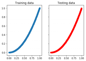
To create some sample data manually, I used 1000 linearly spaced values between 0 and 1. Then shuffled all this data and used the first 500 for training and the other 500 for testing. By doing that, we make sure that test and training data doesn’t overlap and at the same time have a similar distribution. If you look at the scatter plot, they look very much identical but the actual values are 100% different.
For the network part, it is similar to the randomness learning post, but this time I removed one fully connected layer, so now network consists of two weight layers, 1 ReLu activation layer and a MSE loss layer. MSE loss tries to get predicted y value close to the ground truth y value. Here is the network part :
|
1 2 3 4 5 6 7 8 9 10 11 12 13 14 15 16 17 18 19 20 |
#lets first create the tensorflow environment we will work in rng = np.random learning_rate = 0.01 n_samples = train_X.shape[0] X = tf.placeholder(tf.float32, [None, 1]) Y = tf.placeholder(tf.float32, [None, 1]) W1 = tf.Variable(rng.randn(1,128)*2, name="weight1",dtype="float") b1 = tf.Variable(rng.randn(128)*2, name="bias1",dtype="float") fc1 = tf.nn.relu(tf.matmul(X, W1) + b1) W3 = tf.Variable(rng.randn(128,1)*2, name="weight3",dtype="float") b3 = tf.Variable(rng.randn(1)*2, name="bias3",dtype="float") pred = tf.matmul(fc1, W3) + b3 cost = tf.reduce_sum(tf.pow(pred-Y, 2))/(2*n_samples) optimizer = tf.train.GradientDescentOptimizer(learning_rate).minimize(cost) |
Now, after going over my last post, I realized I could add some re-usability to my code. Let’s add a training function which we can use later on to try different models and data. By converting this to a function, this will reduce the copy-paste in the code.
|
1 2 3 4 5 6 7 8 9 10 11 12 13 14 15 16 17 18 19 20 21 22 |
def trainingFunction(sess,optimizer,cost,train_X,train_Y,display_step,training_epochs): loss_history = [] data_count_train = train_X.shape[0] # Fit all training data for epoch in range(training_epochs): for (x, y) in zip(train_X, train_Y): sess.run(optimizer, feed_dict={X: x.reshape([1,1]), Y: y.reshape([1,1])}) c = sess.run(cost, feed_dict={X: train_X.reshape([int(data_count_train),1]), Y:train_Y.reshape([int(data_count_train),1])}) loss_history.append(c) # Display logs per epoch step if epoch % display_step == 0: print("Epoch:", '%04d' % (epoch+1), "cost=", "{:.9f}".format(c)) print("Optimization Finished!") training_cost = sess.run(cost, feed_dict={X: train_X.reshape([int(datacount/2),1]), Y: train_Y.reshape([int(datacount/2),1])}) print("Training cost=", training_cost, '\n') return loss_history |
Now training part:
|
1 2 3 4 5 6 7 8 9 10 11 12 13 14 15 16 17 18 19 20 21 22 23 24 25 26 |
training_epochs = 1000 display_step = 50 #refresh the session and initialize the weights init = tf.global_variables_initializer() sess = tf.Session() sess.run(init) #use the training function we created to train the model loss_history = trainingFunction(sess,optimizer,cost,train_X,train_Y,display_step,training_epochs) plt.plot(loss_history) plt.title('Loss') plt.show() y_res = sess.run(pred, feed_dict={X: train_X.reshape([int(datacount/2),1])}) plt.scatter(train_X,train_Y) plt.scatter(train_X,y_res, color='r') plt.show() y_res_test = sess.run(pred, feed_dict={X: test_X.reshape([int(datacount/2),1])}) plt.scatter(test_X,test_Y) plt.scatter(test_X,y_res_test, color='r') plt.show() |
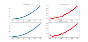
Not bad, I think 🙂 It was a fast and small training, could be improved as well. My most important observation is that the number of neurons in the first layer was very important. It was sort of defining the capacity of the network. When I used 16 neurons in the first layer, I wasn’t able to get that much better results, so be careful with your models and neuron counts.. Another important thing is weight initialization, if you initialize the weights for example with smaller values, they might get stuck at a local minima and not progress further on. So I believe, if you play with the number of neurons, training epoch count and weight initialization; you can get better results than me definitely.
You can find the source code and jupyter notebook version is here in my github : Square function learning code .
I think this is enough for this post for now. If you have questions leave a comment below, I will try to answer. See you in another post, in the meantime keep learning 🙂