Beginner's Guide to R
What is R? “R is a language and environment for statistical computing and graphics. R is an integrated suite of software facilities for data manipulation, calculation and graphical display” from the official website. R is a great tool to have in any Data Scientist’s skill set. It is a statistical and graphical plotting tool more than a programming language.
As I’m learning R myself, I will post what I learned along the way. It is kind of lecture note that might also be helpful to others. I will time to time update this post with more tips and tricks in R. Let’s begin.
Installing R is pretty straightforward. You can find it in the official website after chosing a mirror: https://cran.r-project.org/mirrors.html. After installing and starting R, you will see a command console, similar to how Python works with command shells, you can run any command in the shell, or create scripts and run your scripts through console. I would suggest using RStudio which is like an IDE for R environment. It makes things easier and has a nice interface. It is free for non-commercial use.
<- or -> can be used to assign values to variables. ls() will list the variables(or objects, I think) in memory. Parentheses are essential in R language, if you forget to put parentheses while calling a function, function’s code will be printed. You can use pattern in short pat as a parameter to ls to pick what to display. ; can be used to put multiple codes in one line.
1
2
3
4
a <- 5
ls()     #list data/variables/objects
name <- "yusuf"; myvar <- 23; othervar <- 12
ls(pat = "name")  #will only print name object
To initialize a variable with a sequence of numbers c is used. Indexing is similar to Python but starts from 1. And also in start:end indexing end is included while in Python end is excluded.
1
2
3
4
5
6
7
8
9
10
11
12
13
#create a vector
vc <- c(3,5,7,9,6,8)
vc
[1] 3 5 7 9 6 8

vc[1]
[1] 3

vc[3]
[1] 7

vc[1:3]
[1] 3 5 7
Note that lines starting with [1] are from the console directly, I put them to show what it outputs.
To create sequence of numbers, you can use : or seq. Don’t forget that in R, end is included in start:end syntax.
1
2
3
4
5
6
7
8
9
10
11
12
13
x <- 1:10
x
 [1]  1  2  3  4  5  6  7  8  9 10

seq(1,3,0.5)
 [1] 1.0 1.5 2.0 2.5 3.

seq(from=1,to=3,by = 0.5)
 [1] 1.0 1.5 2.0 2.5 3.0

seq(from=1,to=3,length = 10)
 [1] 1.000000 1.222222 1.444444 1.666667 1.888889 2.111111 2.333333 2.555556
 [9] 2.777778 3.000000
In the last command, [9] indicates that output of the vector at that line starts from 9th element. This makes it easier to understand console outputs, which line contains which elements.
There is also Logical Indexing which is similar to Numpy’s logical indexing. For example to get elements in the vector which are smaller than 5; v[v<5] can be used. v<5 creates a logical vector such as TRUE FALSE FALSE TRUE… And by using this logical vector to index the full vector, we can get the elements smaller than 5 which are logically represented by TRUE in v<5.
Negative indexing is very different from Python and other similar programming languages. In R, negative index stands for deleting/removing the item at that positive index. Note that after negative indexing, actual vector is not modified but a new copy is returned with the negative indexed element removed..
1
2
3
4
5
6
7
8
9
10
11
12
13
v <- c(3,5,1,4,6,8,0)
v[-2]
  [1] 3 1 4 6 8 0        #removed the second element

v
  [1] 3 5 1 4 6 8 0      # v is still same

v <- v[-1]
v
  [1] 5 1 4 6 8 0        #remove 1st element from v and assign it back to v

v[-1:-3]
  [1] 6 8 0              #remove the first 3 elements from v
Functions are declared using assignment operator such as :
1
2
3
4
5
6
7
8
9
10
11
12
13
addAB <- function(a,b)
{
   return(a+b)
}

addAB       #function call without parentheses, will display function code
function(a,b)
{
  return(a+b)
}

addAB(2,6)
  [1] 8
You first declare the code of the function by calling the function function :) This returns a function and it is assigned to the object addAB. Note that if you call addAB without any parentheses, it will only print the function code. Also return is a function and needs to have parentheses. parentheses are essential in R.
It is also possible to use default parameters in functions, syntax is similar to C++.
1
2
3
4
addAB <- function(a, b=10)
{
    return (a+b)
}
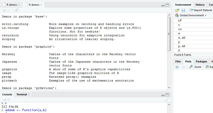
You can use help(function_name) to get detailed information about a function. There are many demo codes that comes with the R environment. To check available demo codes, just type demo(package = .packages(all.available = TRUE)). It will list all available demo codes for all available packages :
Run a demo and check what it does. It will also show the code being executed in console display. To run a code from a specific package : demo(package = “base”,topic = “recursion”).
Last but not least, R has many packages available in: https://cran.r-project.org/web/packages/available_packages_by_name.html. To install packages, to check installed packages or to import a package, you can use these commands:
1
2
3
install.packages("thepackagename")
installed.packages()
library("thepackagename")   # similar to "import package" in python
By the way, there are also some Deep Learning packages, if that rings a bell :)
This covers much of the basic introduction part of the R. I might later on add more to this post, but probably a more intermediate post on R would be more helpful to me and to you. All comments are welcome :) And as always keep learning.
